pythonで軌道シミュレーション
画像書き出し
# Import Python Modules
import numpy as np # 数値計算ライブラリ
import matplotlib.pyplot as plt # 描画ライブラリ
from scipy.integrate import odeint # 常微分方程式を解くライブラリ
# 定数
# G = 6.67430 * 10 **(-20) [km^3 kg^-1 s^-2] 万有引力定数(km)
# M = 5.972 * 10 ** 24 # [kg] 地球質量
GM = 398600 # [km^3 s^-2] 地球の重力定数
# 二体問題の運動方程式
def func(x, t):
r_E = np.linalg.norm([x[0],x[1],x[2]])
dxdt = [x[3],
x[4],
x[5],
-GM*x[0]/(r_E**3),
-GM*x[1]/(r_E**3),
-GM*x[2]/(r_E**3)]
return dxdt
# 微分方程式の初期条件
x0 = [6400, 0, 0, 0, 9, 0] # 位置(x,y,z)+速度(vx,vy,vz)
t = np.linspace(0, 30000, 1000) # (開始、終了、ステップ数) 1日分 軌道伝播
# 微分方程式の数値計算
sol = odeint(func, x0, t)
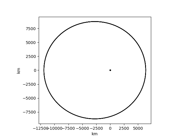
# 二次元描画
fig = plt.figure()
ax = fig.add_subplot(1, 1, 1)
ax.set_xlabel('km')
ax.set_ylabel('km')
#地球をプロット
ax.plot(0,0,'.', c='black') #点をプロットする場合
ax.plot(sol[:, 0],sol[:, 1], 'black') #numpyのnparrayの記法で、各時間の0列目(x座標)、1列目(y座標)を抽出
ax.set_aspect('equal') # グラフのアスペクト比を揃える
plt.savefig('orbit.png') # 画像を保存
plt.show()
kmで計算しているので、万有引力定数が-11乗でなく-20乗になっている。万有引力を万有引力定数Gと地球質量Mから計算すると誤差が大きくなるため、重力定数GMとしてハードコードしている
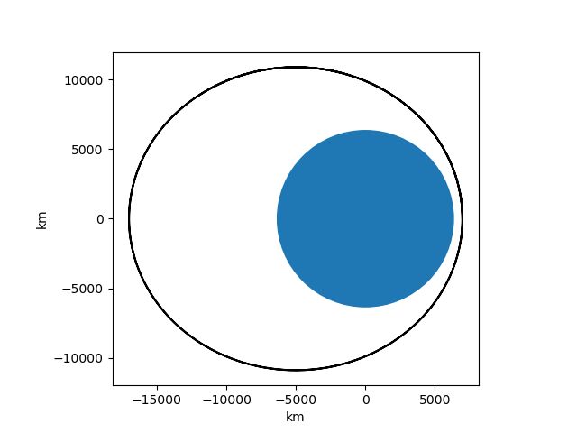
地球の大きさを描画する
# Import Python Modules
import numpy as np # 数値計算ライブラリ
import matplotlib.pyplot as plt # 描画ライブラリ
from scipy.integrate import odeint # 常微分方程式を解くライブラリ
from matplotlib import patches

# 定数
# G = 6.67430 * 10 **(-20) [km^3 kg^-1 s^-2] 万有引力定数(km)
# M = 5.972 * 10 ** 24 # [kg] 地球質量
GM = 398600 # [km^3 s^-2] 地球の重力定数
R = 6378
# 二体問題の運動方程式
def func(x, t):
    r_E = np.linalg.norm([x[0],x[1],x[2]])
    dxdt = [x[3],
            x[4],
            x[5],
            -GM*x[0]/(r_E**3),
            -GM*x[1]/(r_E**3),
            -GM*x[2]/(r_E**3)]
    return dxdt

# 微分方程式の初期条件
x0 = [R+600, 0, 0, 0, 9, 0] # 位置(x,y,z)+速度(vx,vy,vz)
t  = np.linspace(0, 30000, 1000) # (開始、終了、ステップ数) 1日分 軌道伝播

# 微分方程式の数値計算
sol = odeint(func, x0, t)

# 二次元描画
fig = plt.figure()
ax = fig.add_subplot(1, 1, 1)
ax.set_xlabel('km')
ax.set_ylabel('km')

#地球をプロット
c = patches.Circle( (0,0), R)
ax.add_patch(c)
# ax.plot(0,0,'.') #点をプロットする場合

ax.plot(sol[:, 0],sol[:, 1], 'black') #numpyのnparrayの記法で、各時間の0列目(x座標)、1列目(y座標)を抽出
ax.set_aspect('equal') # グラフのアスペクト比を揃える
plt.savefig('orbit.png') # 画像を保存
plt.show()
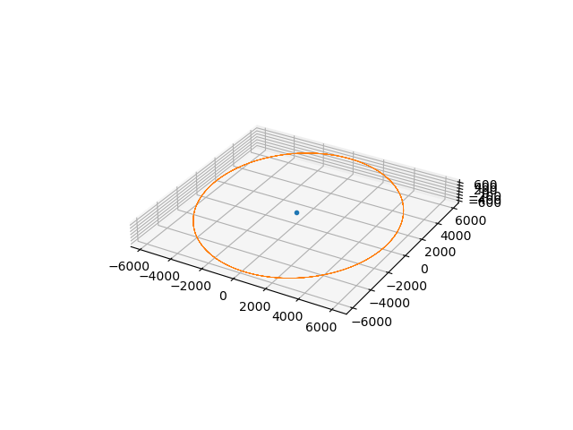
マウスを使って三次元で観察する
# Import Python Modules
import numpy as np # 数値計算ライブラリ
import matplotlib.pyplot as plt # 描画ライブラリ
from scipy.integrate import odeint # 常微分方程式を解くライブラリ

# 定数
# G = 6.67430 * 10 **(-20) [km^3 kg^-1 s^-2] 万有引力定数(km)
# M = 5.972 * 10 ** 24 # [kg] 地球質量
GM = 398600 # [km^3 s^-2] 地球の重力定数

# 二体問題の運動方程式
def func(x, t):
    r_E = np.linalg.norm([x[0],x[1],x[2]])
    dxdt = [x[3],
            x[4],
            x[5],
            -GM*x[0]/(r_E**3),
            -GM*x[1]/(r_E**3),
            -GM*x[2]/(r_E**3)]
    return dxdt

# 微分方程式の初期条件
x0 = [6000, 0, 0, 0, 8, 1] # 位置(x,y,z)+速度(vx,vy,vz)
t  = np.linspace(0, 30000, 1000) # (開始、終了、ステップ数) 1日分 軌道伝播

# 微分方程式の数値計算
sol = odeint(func, x0, t)

# 三次元描画
fig = plt.figure()
ax = fig.add_subplot(1, 1, 1, projection='3d')
ax.plot(0,0,0,'.')#地球をプロット
ax.plot(sol[:, 0], sol[:, 1], sol[:, 2],linewidth = 0.5)
ax.set_aspect('equal') # グラフのアスペクト比を揃える
plt.show()
初速のz成分を0km/sから1km/sに変更し、三次元でプロットした
gif動画を書き出す
import numpy as np
import matplotlib.pyplot as plt
import matplotlib.animation as animation
from scipy.integrate import odeint # 常微分方程式を解くライブラリ


GM_E = 398600 # km3/s2 地球の重力定数
L_E = [0,0,0]

def func(x, t):
    r_E = np.linalg.norm([x[0]-L_E[0],x[1]-L_E[1],x[2]-L_E[2]])
    dxdt = [x[3],
            x[4],
            x[5],
            -GM_E*x[0]/(r_E**3),
            -GM_E*x[1]/(r_E**3),
            -GM_E*x[2]/(r_E**3)]
    return dxdt

def update(i, x, y):

    plt.plot(x[0:i], y[0:i],c="blue")

def draw():
    # 微分方程式の初期条件
    r0 = [6500, 0, 0, 0, 9, 0] # 位置(x,y,z)+速度(vx,vy,vz)
    t  = np.linspace(0, 10000, 1000) # 1日分 軌道伝播
    sol = odeint(func, r0, t)
    print("keisan owari")

    # 抽出して二次元化
    x1, y1, z1 = sol[:, 0], sol[:, 1], sol[:, 2]
    x = x1[::10]
    y = y1[::10]

    fig = plt.figure() #figure objectを取得
    plt.plot(0,0,'.',c='blue')# 地球をプロット
    plt.xlim(min(x),max(x))
    plt.ylim(min(y),max(y))
    plt.gca().set_aspect('equal')

    ani = animation.FuncAnimation(fig, update, fargs = (x, y), frames = len(x),interval = 10)
    ani.save("orbit.gif", writer = 'pillow',fps=30)
draw()
mp4を書き出す
mp4を書き出す場合は、writerをpillowから次のように変える
    ani = animation.FuncAnimation(fig, update, fargs = (x, y), frames = len(x),interval = 10)
    writer = animation.writers['ffmpeg'](fps=60, metadata=dict(artist='mika'), bitrate=200)
    ani.save("orbit.mp4", writer = writer)
月と、太陽の摂動と、太陽地球回転フレーム
import numpy as np
import matplotlib.pyplot as plt
import matplotlib.animation as animation
from scipy.integrate import odeint # 常微分方程式を解くライブラリ
import glob

# G = 6.67430 * 10 **(-11) [m3 kg-1 s-2] 万有引力定数(mksa)
# G = 6.67430 * 10 **(-20) [km3 kg-1 s-2] 万有引力定数(km)

# ME = 5.972 * 10 ** 24 # [kg] 地球質量
# MM = 7.345 * 10 ** 22 # [kg] 月質量
MS = 1.989 * 10 ** 30 # [kg] 太陽質量

GM_E = 398600.4354360959 # [km3 s-2] 地球の重力定数
GM_M = 4902.8072 # [km3/s2] 月の重力定数
GM_S = 13.27 * 10 ** 10 # [km3 s-2] 太陽の重力定数

L_E = [0,0,0] # 地球の座標[km]

# R_SE = 1.496 * 10 ** 8 # [km] 地球公転半径
R_EM = 3.8 * 10 ** 5 # [km] 月公転半径

# A = 5.927 * 10 ** -6 # [km s-2] 地球付近での太陽重力の加速度
# GM_S/R_SE
W = 2*np.pi/(86400*365)
w = 2*np.pi/(86400*30)
gradA = 17.74 * 10 ** (-14) # GM_S/R_SE ** 3 # [km s-2] 地球付近での太陽重力と遠心力による加速度の傾斜  GM_S/R_SE**2 + W**2

def L_M(t):
    # 月の運動
    offset = 170/360 * 2*np.pi
    return [-384400*np.cos(w*t+offset),-384400*np.sin(w*t+offset),0]

def F(r, t):
    r_E = np.linalg.norm([r[0]-L_E[0],r[1]-L_E[1],r[2]-L_E[2]])
    r_M = np.linalg.norm([r[0]-L_M(t)[0],r[1]-L_M(t)[1],r[2]-L_M(t)[2]])
    LM = L_M(t)

    dxdt = [r[3],
            r[4],
            r[5],
            GM_E*(L_E[0]-r[0])/(r_E**3) + GM_M*(LM[0]-r[0])/(r_M**3) + gradA * r[0] * np.cos(W*t),
            GM_E*(L_E[1]-r[1])/(r_E**3) + GM_M*(LM[1]-r[1])/(r_M**3) + gradA * r[1] * np.sin(W*t),
            GM_E*(L_E[2]-r[2])/(r_E**3) + GM_M*(LM[2]-r[2])/(r_M**3)]
    return dxdt

def update(i, x, y, unittime,framew):
    t = i*unittime
    LM = L_M(t)
    plt.cla() #現在描写されているグラフを消去
    plt.plot(0,0,0,'.',c='blue')# 地球をプロット
    plt.plot(LM[0]*np.cos(framew*t)+LM[1]*np.sin(framew*t),
             -LM[0]*np.sin(framew*t)+LM[1]*np.cos(framew*t),
             '.',c='red')# 月をプロット
    plt.xlim(-2000000,1500000)
    plt.ylim(-1500000,1500000)

    plt.plot(x[0:i], y[0:i],c="blue") #plot
    plt.text(-1500000,-1000000,f'day = {int(t/86400)}', fontsize=10)

def draw():
    # 微分方程式の初期条件r0
    v0 = 11.48964 #初速12.5922 12.592
    h0 = 6000 # 初期高度
    th0 = np.pi*1 # 初期位置の経度(太陽側が0、反時計回り)
    r0 = [-h0*np.cos(th0), -h0*np.sin(th0), 0, v0*np.sin(th0), -v0*np.cos(th0), 0] # 位置[km](x,y,z)+速度[km/s](vx,vy,vz)

    # 微分方程式の計算設定
    timeRange = int(86400 * 320) #時間範囲[s] (参考 1d=86400s)
    calcStep = 40 #時間ステップ[s]
    t  = np.linspace(0, timeRange, int(timeRange/calcStep)) # 時間範囲(開始[s],終了[s],分割数)

    # 微分方程式を解く
    sol = odeint(F, r0, t) # [x, y, z, u, v, w]

    # print(sol[5])
    x1 = []
    y1 = []
    z1 = []

    framew = W

    for i, raw in enumerate(sol):
        t = i*calcStep
        x1.append(raw[0]*np.cos(framew*t) + raw[1]*np.sin(framew*t))
        y1.append(-raw[0]*np.sin(framew*t) + raw[1]*np.cos(framew*t))
        z1.append(raw[2])

    # 動画保存用にフレームを抜き出す
    skiprate = int(1440/calcStep*15) #144skiprateで、60fps 10秒step計算で1秒が一日になる
    x = x1[::skiprate]
    y = y1[::skiprate]

    dic = calcStep*skiprate

    fig = plt.figure() #figure objectを取得
    plt.gca().set_aspect('equal')

    ani = animation.FuncAnimation(fig, update, fargs = (x, y,dic,framew), frames = len(x),interval = 10)

    # savemp4(ani,'ww.mp4')
    savegif(ani,'16.gif')
    # savemp4(ani,getname())

def getname():
    filelist = [int(filename.split('.')[0].replace('test','')) for filename in glob.glob('*.mp4')]
    return f'test{max(filelist)+1}.mp4'

def savemp4(ani,filename):
    writer = animation.writers['ffmpeg'](fps=60, metadata=dict(artist='mika'), bitrate=200)
    ani.save(filename, writer = writer)

def savegif(ani,filename):
    ani.save(filename, writer = 'pillow', fps=30)

draw()